
8주차: 5월 25일 ~ 5월 29일
멀티캠퍼스 부트캠프 8주차 요약✍️
[ 5/25 ] 대체공휴일 휴강
[ 5/26 ] 딥러닝: RNN, LSTM_회귀
[ 5/27 ] 딥러닝: LSTM_분류
[ 5/28 ] 투자 전략: Bollinger Band, BuyandHold
[ 5/29 ] 투자 전략: Momentum
5월 26일👩🏻💻
오늘의 소감: 틀리면서 배우는 딥~러~닝~
학습률 0.001을 0.01로 바꾸니까 MSE 진짜 난리나던데 하...🫠
0 하나를 못봐서 점심시간 내내 코드를 보고 있었다.
💻 RNN
AAPL(애플 주식) 데이터 활용
라이브러리, 데이터 로드
import pandas as pd
import matplotlib.pyplot as plt
import torch
import torch.nn as nn
import torch.optim as optim
from torch.utils.data import Dataset, DataLoader
from sklearn.preprocessing import StandardScaler, MinMaxScaler
from sklearn.metrics import mean_squared_error, r2_score

df = pd.read_csv("../csv/aapl.csv")
df.info()
데이터 전처리
df.dropna(inplace=True)

df = df[['Date', 'Adj Close']]
values = df[['Adj Close']].values

df['Adj Close'].values.reshape(-1, 1)

split_idx = int(len(values) * 0.75)

train_data = values[:split_idx]
test_data = values[split_idx:]

# MinMaxScaler로 데이터 정규화
scaler = MinMaxScaler()
train_sc = scaler.fit_transform(train_data)
test_sc = scaler.transform(test_data)

# 스케일링이 완료된 데이터를 Tensor로 변환
train_sc = torch.tensor(train_sc, dtype=torch.float32)
test_sc = torch.tensor(test_sc, dtype=torch.float32)
Dataset 생성, DataLoader 사용을 통한 train_dl/test_dl 생성
class WindowDataset(Dataset):
    def __init__(self, _data, _window):
        # _data : tensor, array 1차원 데이터 형태
        # _window : 구간의 크기
        self.data = _data
        self.window = _window
        # DataLoader에서 사용 가능한 인덱스의 최대 값
        self.n = len(_data) - _window

    def __len__(self):
        return self.n

    def __getitem__(self, idx):
        # idx : 0 ~ self.n-1 사이의 정수가 대입 (DataLoader에서 자동으로 대입)
        x = self.data[idx:idx + self.window]
        y = self.data[idx + self.window]
        return x, y

# WindowDataset에 데이터를 대입
train_ds = WindowDataset(train_sc, _window=60)
test_ds = WindowDataset(test_sc, _window=60)

# Dataset를 DataLoader로 생성
train_dl = DataLoader(train_ds, batch_size=128, shuffle = True, drop_last = True)
test_dl = DataLoader(test_ds, batch_size=256, shuffle=False, drop_last = False)
RNN Model, 검증 데이터 평가 함수 생성
RNN Model
# RNN 모델 정의
class RNNModel(nn.Module):
    def __init__(self,
                 input_size,
                 hidden_size = 64,
                 num_layers = 1,
                 dropout = 0.0,
                 nonlinearity = 'tanh',
                 bidirectional = False):
        super(RNNModel, self).__init__()
        # super().__init__()
        self.rnn = nn.RNN(
            input_size = input_size,
            hidden_size = hidden_size,
            num_layers = num_layers,
            dropout = dropout,
            nonlinearity = nonlinearity,
            bidirectional = bidirectional,
            # batch_first가 False인 경우, 입력 데이터(구간의 개수, 배치크기, 입력 데이터 피쳐의 수)
            # (배치 크기, 구간의 크기, 입력 피쳐의 개수) --> True로 변경
            batch_first = True
        )

        # output_feature가 역방향을 포함한다면 2배로 늘어난다.
        if bidirectional:
            hidden_size *= 2
        print(f"hidden_size : {hidden_size}")
        self.model = nn.Linear(hidden_size, 1)


    def forward(self, x):
        out, h_n = self.rnn(x)
        last_hidden = h_n[-1]
        result = self.model(last_hidden)
        return result
# 모델 학습 시 검증 데이터를 이용하여 모델의 성능을 평가 할수 있도록 검증 데이터 평가 함수
@torch.no_grad()
def evaluate_mse(dataloader, model):
# dataloader -> 검증 데이터셋의 dataloader
model.eval()
total_loss = 0
total_n = 0
for x, y in dataloader:
x = x.float()
y = y.float()
pred = model(x)
loss = nn.MSELoss()(pred, y)
total_loss += loss.item() * x.size(0)
total_n += x.size(0)
return total_loss / max(total_n, 1)RNN Model 호출, 평가 지표, optimizer 생성
aapl_model = RNNModel(
    input_size = 1,
    hidden_size = 128
)

criterion = nn.MSELoss()
optimizer = optim.Adam(aapl_model.parameters(), lr = 0.001)		# 문제의 0.01과 0.001...
train_history, test_history = [], []
for epoch in range(20):
aapl_model.train()
running, n_seen = 0.0, 0
for x, y in train_dl:
x = x.float()
y = y.float()
pred = aapl_model(x)
loss = criterion(pred, y)
optimizer.zero_grad()
loss.backward()
# 가중치 발산 방지
nn.utils.clip_grad_norm_(aapl_model.parameters(), 1.0)
optimizer.step()
running += loss.item() * y.size(0)
n_seen += y.size(0)
train_mse = running / n_seen
test_mse = evaluate_mse(test_dl, aapl_model)
train_history.append(train_mse)
test_history.append(test_mse)
print(f"Epoch {epoch+1} Train MSE: {round(train_mse, 8)} Test MSE: {round(test_mse, 8)}")
시각화
aapl_model.eval()		# 평가 모드

preds = []
trues = []

with torch.no_grad():
    for x, y in test_dl:
        x = x.float()
        y = y.float()

        pred = aapl_model(x)
        preds.append(pred.cpu())
        trues.append(y.cpu())


# cat 함수: pd.concat() 과 같은 역할
preds = torch.cat(preds, dim=0).squeeze(-1).numpy()
trues = torch.cat(trues, dim=0).squeeze(-1).numpy()


# 시각화
plt.figure(figsize = (14, 10))
plt.plot(preds[:600], label = 'Preds')
plt.plot(trues[:600], label = 'Trues')
plt.legend()
plt.grid()
plt.show()
💻 LSTM
AAPL 데이터 활용
코드는 RNN과 매우 유사하지만, 예측값을 2개 돌려주는 RNN과 달리 LSTM은 3개를 돌려준다.
또한 nn.LSTM에는 nn.RNN에 없는 head_type이라는 인자가 존재한다.
라이브러리
import pandas as pd
import matplotlib.pyplot as plt
import torch
import torch.nn as nn
import torch.optim as optim

from torch.utils.data import Dataset, DataLoader
from sklearn.preprocessing import MinMaxScaler
from sklearn.model_selection import train_test_split
함수화를 위한 작업
# 하나의 함수화
# 매개변수로 사용할 데이터들은 어떤 것이 있을까?

# 파일의 경로를 지정하는 변수 (read_csv)
file_path = '../csv/aapl.csv'

# 구간(window) 설정 (Dataset)
window = 60

# batch size 지정 (DataLoader)
x_batch = 64
y_batch = 256

# 기여도 (optimizer)
lr = 0.001

# 반복 학습 횟수
epochs = 20

# 은닉층에서의 뉴런(feature)의 개수
hidden_cnt = 64

# Layer 설정값
layer_cnt = 1

# train, test 비율
train_ratio = 0.8

# 은닉층, 셀 구조에서 어떤 부분을 사용할 것인가?
    # 'h': 은닉층 사용 // 'c': 셀 사용 // 'h_c': 둘 다 사용
head_type = 'h_c'
데이터 로드, 전처리
df = pd.read_csv(file_path)
df.dropna(inplace=True)

df['Date'] = pd.to_datetime(df['Date'])
X = df[['Adj Close', 'Volume']].astype(float).values
y = df[['Adj Close']].astype(float).values

X_train, X_test, y_train, y_test = train_test_split(
    X, y, train_size = train_ratio, shuffle = False
)

scaler_x = MinMaxScaler()
scaler_y = MinMaxScaler()

X_train_sc = scaler_x.fit_transform(X_train)
X_test_sc = scaler_x.transform(X_test)
y_train_sc = scaler_y.fit_transform(y_train)
y_test_sc = scaler_y.transform(y_test)
Dataset 생성, DataLoader 사용을 통한 train_dl/test_dl 생성
class WindowDataset(Dataset):
    def __init__(self, _x, _y, _window):
        self.x = _x
        self.y = _y
        self.window = _window
        self.n = (len(_x) - _window)

    def __len__(self):
        return max(self.n, 1)

    def __getitem__(self, idx):
        x = self.x[idx  :  idx + self.window]
        y = self.y[idx + self.window]
        x_tensor = torch.tensor(x, dtype = torch.float32)
        y_tensor = torch.tensor(y, dtype = torch.float32)
        return x_tensor, y_tensor

train_ds = WindowDataset(X_train_sc, y_train_sc, window)
test_ds = WindowDataset(X_test_sc, y_test_sc, window)

train_dl = DataLoader(train_ds, shuffle = True, drop_last = True, batch_size = x_batch)
test_dl = DataLoader(test_ds, shuffle = False, drop_last=False, batch_size = y_batch)
LSTM 정의
class LSTMModel(nn.Module):

    def __init__(
            self,
            input_size,
            hidden_size = 64,
            num_layers = 1,
            dropout = 0.0,
            bidirectional = False,
            batch_first = True,
            head_type = 'h'
    ):
        super(LSTMModel, self).__init__()

        # LSTM 기본 설정
        self.lstm = nn.LSTM(
            input_size = input_size,
            hidden_size = hidden_size,
            num_layers = num_layers,
            dropout = dropout,
            bidirectional = bidirectional,
            batch_first = batch_first
        )

        # bidirectional이 True면 out feature의 개수가 2배
        hidden_size = hidden_size * (2 if bidirectional else 1)

        # head_type에 따라서 출력의 feature 개수가 달라진다.
        if head_type in ['h', 'c']:
        #if (head_type == 'h') | (head_type == 'c')
            pass
        elif head_type == 'h_c':
            hidden_size = hidden_size * 2
        else:
            print('head_type의 인자값을 잘못 입력하였습니다. ("h", "c", "h_c")를 사용해주세요')

        # 선형 모델 생성
        self.model = nn.Linear(hidden_size, 1)
            # 객체 안에 독립적인 데이터를 저장
        self.head_type = head_type

    # 순전파 함수 정의
    def forward(self, x):
        # 순전파의 예측값 (RNN은 2개를 되돌려줌, LSTM은 3개를 되돌려줌)
        out, (h_n, c_n) = self.lstm(x)
        # 은닉층의 가장 마지막값 저장
        h_last = h_n[-1]
        c_last = c_n[-1]

        if self.head_type == 'h':
            feat = h_last
        elif self.head_type == 'c':
            feat = c_last
        elif self.head_type == 'h_c':
            feat = torch.cat([h_last, c_last], dim = -1)

        return self.model(feat)
여기서 __init__ 함수에 들어간 parameter들은 기본값으로 사용될 것이다.
모델 생성
model = LSTMModel(input_size = 2, hidden_size = hidden_cnt, head_type = head_type)
model
손실 함수, 옵티마이저 정의
criterion = nn.MSELoss()
optimizer = optim.Adam(model.parameters(), lr = lr)
평가 함수 생성
# 검증 데이터의 loss값 확인하는 함수

# @torch.no_grad()
def evaluate_mse(dl):
    model.eval()

    total_loss, total_n = 0.0, 0
    # 데코레이터 또는 여기 사용
    with torch.no_grad():
        for x, y in dl:
            x = x.float()
            y = y.float()
            pred = model(x)
            loss = criterion(pred, y)
            total_loss += loss.item() * y.size(0)
            total_n += y.size(0)

    return total_loss / max(total_n, 1)
반복 학습
# 반복 학습

test_history = []

for epoch in range(epochs):
    model.train()

    total_loss, total_n = 0.0, 0

    for x, y in train_dl:
        x = x.float()
        y = y.float()

        pred = model(x)
        loss = criterion(pred, y)

        optimizer.zero_grad()
        loss.backward()
        # 기울기 발산 방지 (이 자리 아니면 소용 없음)
        nn.utils.clip_grad_norm_(model.parameters(), 1.0)
        optimizer.step()

        total_loss += loss.item() * y.size(0)
        total_n += y.size(0)

    train_loss = total_loss / max(total_n, 1)
    test_loss = evaluate_mse(test_dl)
    test_history.append(test_loss)
    print(f"Epoch: {epoch+1}, train_mse: {round(train_loss, 4)}, test_mse: {round(test_loss, 4)}")
간단 시각화
# test_history를 그래프로 시각화

plt.plot(test_history)
plt.show()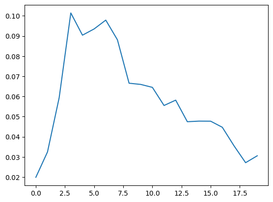
예측값 생성
model.eval()

preds, trues = [], []

with torch.no_grad():
    for x, y in test_dl:
        x = x.float()
        pred = model(x)
        preds.append(pred)
        trues.append(y)

# tensor 데이터들을 하나로 합쳐주고 차원을 벗겨낸 다음 array로 변환
preds = torch.cat(preds, dim=0).numpy()
trues = torch.cat(trues, dim=0).numpy()

# 스케일링 데이터를 원본 데이터로 변환
pred_origin = scaler_y.inverse_transform(preds).squeeze(-1)
true_origin = scaler_y.inverse_transform(trues).squeeze(-1)
시각화
plt.figure(figsize = (16, 10))
plt.plot(pred_origin, label = 'Pred Origin')
plt.plot(true_origin, label = 'True Origin')

plt.legend()
plt.grid()
plt.xlabel('Date')
plt.ylabel('Adj Close')

plt.show()
5월 27일👩🏻💻
오늘의 소감: 시간이 순식간에 흘러간다... 분명 한 건 많지 않은 것 같은데 뇌에 과부하가 걸려서 진행을 못 하는 느낌🫠
💻 LSTM_분류
날씨 데이터 활용
라이브러리, 데이터 로드
import pandas as pd
import numpy as np
import requests
import torch
import torch.nn as nn
import torch.optim as optim
import matplotlib.pyplot as plt
import platform

from sklearn.metrics import accuracy_score
from torch.utils.data import Dataset, DataLoader
from sklearn.preprocessing import MinMaxScaler

---

url = "https://archive-api.open-meteo.com/v1/archive"

params = {
    'latitude': 37.5665,
    'longitude': 126.9780,
    'start_date': '2025-01-01',
    'end_date': '2025-12-31',
    'hourly': 'temperature_2m,relative_humidity_2m,surface_pressure,wind_speed_10m,rain'
}

res = requests.get(url, params = params)
data = res.json()


# 날씨 데이터들을 따로 추출
df = pd.DataFrame(data['hourly'])
df.columns = ['측정 시간', '기온', '상대 습도', '지면 기압', '풍속', '강수량']
데이터 전처리
x = df[['기온', '상대 습도', '지면 기압', '풍속']].values
y = df['target'].values

x_sc = MinMaxScaler().fit_transform(x)
Dataset 생성, DataLoader 사용 train_dl/test_dl 생성
class windowDS(Dataset):
    def __init__(self, _x, _y, _window):
        self.x = _x
        self.y = _y
        self.window = _window
        self.n = len(_x) - _window

    def __len__(self):
        return self.n

    def __getitem__(self, idx):
        x = self.x[ idx : idx + self.window ]
        y = self.y[ idx + self.window ]
        x_tensor = torch.tensor(x).float()
        y_tensor = torch.tensor(y).long()

        return x_tensor, y_tensor

window = 72
train_ds = windowDS(x_sc, y, window)
train_dl = DataLoader(train_ds, batch_size = 64, shuffle=False)
LSTM 모델 생성
class LSTMclf(nn.Module):
    def __init__(
            self,
            input_size,
            hidden_size
    ):
        super(LSTMclf, self).__init__()
        self.lstm = nn.LSTM(
            input_size = input_size,
            hidden_size = hidden_size,
            batch_first = True
        )
        self.model = nn.Linear(hidden_size, 2)

    def forward(self, x):
        out, (h_n, c_n) = self.lstm(x)
        # h_n[-1], c_n[-1]: bidirectional이 False인 경우 사용 가능
            # True인 경우 역방향의 아웃풋 피쳐만 불러온다.
        # out: 3차원 데이터셋 → [batch, window, feature]
        # 2차원 데이터셋의 형태로 변경 → out[:, -1, :] → [batch, feature]
        pred = self.model(out[:, -1, :])
        return pred
모델 정의, 손실 함수, 옵티마이저 생성
model = LSTMclf(input_size = x.shape[1], hidden_size=32)
criterion = nn.CrossEntropyLoss()
optimizer = optim.Adam(model.parameters(), lr=0.001)
반복 학습
model.train()

for epoch in range(20):
    total_loss, total_n = 0.0, 0
    current1 = current2 = 0
    acc_list = []

    for x, y in train_dl:
        res = model(x)
        loss = criterion(res, y)
        optimizer.zero_grad()
        loss.backward()
        nn.utils.clip_grad_norm_(model.parameters(), 1.0)
        optimizer.step()

        total_loss += loss.item()
        total_n += y.size(0)
        _, pred = torch.max(res, 1)
        acc = accuracy_score(y.numpy(), pred.numpy())
        acc_list.append(acc)

        current1 += (y == pred).sum().item()

    train_loss = total_loss / len(train_dl)
    mean_current = (current1 / max(total_n, 1)) * 100
    current2 = np.mean(acc_list)

    print(f'Epoch: {epoch+1}, EntropyLoss: {round(train_loss, 3)}, \
    Acc1: {round(mean_current, 3)}, Acc2: {round(current2, 3)}')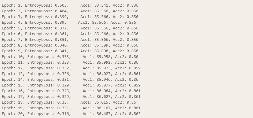
예측
model.eval()

eval_loader = DataLoader(train_ds, batch_size = 1000, shuffle=False)

# 첫번째 데이터만 로드
x, y = next(iter(eval_loader))

with torch.no_grad():
    test_out = model(x)
    _, test_pred = torch.max(test_out, 1)
시각화
# 한글 인코딩을 위해
if platform.system() == 'Windows':
    plt.rc('font', family = 'Malgun Gothic')

plt.rcParams['axes.unicode_minus'] = False

# 시각화
plt.figure(figsize=(15, 5))
plt.plot(y.numpy(), label = '실제 강수 여부', color = 'gray', drawstyle = 'steps-mid', alpha = 0.5)
plt.plot(test_pred.numpy(), label = 'LSTM의 결과', color = 'blue', linestyle = '--', drawstyle = 'steps-mid', alpha=0.7)
plt.yticks([0, 1], ['맑음(0)', '비(1)'])
plt.legend()
plt.show()
5월 28일👩🏻💻
오늘의 소감: 클래스 지옥😵
💻 Bollllinger Band
Amazon 주식 데이터(AMZN) 활용
라이브러리, 데이터 로드
import pandas as pd
import numpy as np
import matplotlib.pyplot as plt
from datetime import datetime

df = pd.read_csv('../csv/AMZN.csv', index_col = 'Date')
df.head()
데이터 전처리, 파생 변수 생성
flag = df.isin( [np.nan, np.inf, -np.inf] ).any(axis = 1)
df = df.loc[~flag, ]

# 종가 이외의 데이터를 제외
df = df[['Adj Close']]

# 이동평균선 → rolling
df['center'] = df['Adj Close'].rolling(20).mean()

# 상단 밴드, 하단 밴드 생성
std_value = 2 * df['Adj Close'].rolling(20).std()
df['ub'] = df['center'] + std_value
df['lb'] = df['center'] - std_value

# index 값을 시계열로 변경
df.index = pd.to_datetime(df.index)

# 투자 시작 시간 설정
start = '2010-01-01'
test_df = df.loc[start: , ]
test_df.head()
보유 내역 추가
# 구매 상태를 입력할 수 있는 공간 생성

test_df['trade'] = ''
test_df.head()
상단 밴드보다 수정 주가가 높거나 같은 경우인데 현재 보유 중: 매도
상단 밴드보다 수정 주가가 높거나 같은 경우인데 보유 중 아님: 유지
하단 밴드보다 수정 주가가 낮거나 같은 경우인데 현재 보유 중: 유지
하단 밴드보다 수정 주가가 낮거나 같은 경우인데 보유 중 아님: 매수
수정 주가가 밴드 사이에 존재하는 경우인데 현재 보유 중: 유지
수정 주가가 밴드 사이에 존재하는 경우인데 보유 중 아님: 유지
for i in test_df.index:

    # 상단 밴드보다 수정 종가가 높은 경우
    if test_df.loc[i, 'Adj Close'] >= test_df.loc[i, 'ub']:
        # 보유 중이라면 trade = '', 아니라면 trade = ''
        test_df.loc[i, 'trade'] = ''

    # 하단 밴드보다 수정 종가가 낮은 경우
    elif test_df.loc[i, 'Adj Close'] <= test_df.loc[i, 'lb']:
        # 보유 중이라면 trade = 'buy', 아니라면 trade = 'buy'
        test_df.loc[i, 'trade'] = 'buy'

    else:
        # 보유 중인 경우 trade = 'buy', 보유 중이 아니면 trade = ''
        # 전날의 trade가 buy인 경우: 보유 중
        if test_df.shift().loc[i, 'trade'] == 'buy':
            test_df.loc[i, 'trade'] = 'buy'
        else:
            test_df.loc[i, 'trade'] = ''
수익률 계산
# 수익률 column 생성, 1로 채워준다

test_df['rtn'] = 1.0
for i in test_df.index:
# 매수 가격 형성
if (test_df.shift().loc[i, 'trade'] == '') & (test_df.loc[i, 'trade'] == 'buy'):
buy = test_df.loc[i, 'Adj Close']
print(f'매수일: {i}, 매수가: {buy}')
# 매도 가격 형성
elif (test_df.shift().loc[i, 'trade'] == 'buy') & (test_df.loc[i, 'trade'] == ''):
sell = test_df.loc[i, 'Adj Close']
# 수익률 계산
rtn = sell / buy
test_df.loc[i, 'rtn'] = rtn
print(f'매도일: {i}, 매도가: {sell}, 수익률: {rtn}')
누적 수익률 계산 → rtn 누적곱
acc_rtn = 1.0

for i in test_df.index:
    rtn = test_df.loc[i, 'rtn']
    acc_rtn *= rtn

test_df['acc_rtn'] = test_df['rtn'].cumprod()
test_df.iloc[-1, -1]
	# np.float64(3.138061358619031)
번외: Buy and Hold
계산이 간단해서 제목을 따로 사용하진 않은 Buy and Hold...
# 투자 기간 첫날 → 매수가
# 투자 마지막 날 → 매도가

bnh_rtn = test_df.iloc[-1, 0] / test_df.iloc[0, 0]
print(bnh_rtn)
	# 14.249095911087196
💻 함수화
지금까지 만든 것들을 매개변수를 통일하여 하나의 클래스 속 3개의 함수로 연결짓는 과정
def create_band(
        _df,
        _col = 'Adj Close',
        _start = '2010-01-01',
        _end = datetime.now(),
        _cnt = 20
):

    df = _df.copy()

    if 'Date' in df.columns:
        df.set_index('Date', inplace=True)

    df.index = pd.to_datetime(df.index)

    df.index = df.index.tz_localize(None)

    flag = df.isin( [ np.nan, np.inf, -np.inf ] ).any(axis=1)
    df = df.loc[~flag, ]

    df = df[[_col]]

    df['center'] = df[_col].rolling(_cnt).mean()

    std_value = 2 * df[_col].rolling(_cnt).std()
    df['ub'] = df['center'] + std_value
    df['lb'] = df['center'] - std_value

    df = df.loc[_start:_end, ]

    return df
df2 = pd.read_csv('../csv/aapl.csv')
band_df = create_band2(df2)2. 보유 내역 생성 함수
def create_trade(_df):
    # 기준 컬럼 이름을 어떻게 알 것인가?: 첫번째 함수의 return으로 나온 df의 첫번째 컬럼만
    col = _df.columns[0]
    df = _df.copy()
    df['trade'] = ''

    for i in df.index:
        if df.loc[i, col] >= df.loc[i, 'ub']:
            # 매도
            df.loc[i, 'trade'] = ''
        elif df.loc[i, col] <= df.loc[i, 'lb']:
            # 매수
            df.loc[i, 'trade'] = 'buy'
        else:
            if df.shift().loc[i, 'trade'] == 'buy':
                df.loc[i, 'trade'] = 'buy'
            else:
                df.loc[i, 'trade'] = ''

    return df
trade_df = create_trade(band_df)3. 수익률 계산 함수
def create_rtn(_df):
    col = _df.columns[0]
    df = _df.copy()

    df['rtn'] = 1.0

    # 수익률 계산
    for i in df.index:
        # 매수
        if (df.shift().loc[i, 'trade'] == '') & (df.loc[i, 'trade'] == 'buy'):
            buy = df.loc[i, col]
            print(f"매수일: {i}, 매수가: {buy}")
            print()
        elif (df.shift().loc[i, 'trade'] == 'buy') & (df.loc[i, 'trade'] == ''):
            sell = df.loc[i, col]
            rtn = sell / buy
            df.loc[i, 'rtn'] = rtn
            print(f"매도일: {i}, 매도가: {sell}, 수익률: {rtn}")
            print()
    # 누적 수익률
    df['acc_rtn'] = df['rtn'].cumprod()
    # 최종 수익률
    acc_rtn = df.iloc[-1, -1]

    return df, acc_rtn
rtn_df, acc_rtn = create_rtn(trade_df)
acc_rtn		# np.float64(1.3923287814461949)
rtn_df
Class로 묶기
class Investing():
    def __init__(self, _df, _col = 'Adj Close', _start = '2010-01-01', _end = datetime.now()):
        self.df = _df
        self.col = _col
        self.start = _start
        self.end = _end

    # 바이앤홀드 함수
    def bnh(self):
        df = self.df.copy()
        if 'Date' in df.columns:
            df.set_index('Date', inplace=True)
        df.index = pd.to_datetime(df.index)
        df = df.loc[self.start:self.end, [self.col]]
        buy = df.iloc[0, 0]
        sell = df.iloc[-1, 0]
        return sell / buy

    # 볼린져 밴드 함수
    def boll(self, _cnt = 20):
        band_df = create_band(self.df, self.col, self.start, self.end, _cnt)
        trade_df = create_trade(band_df)
        rtn_df, acc_rtn = create_rtn(trade_df)
        return rtn_df, acc_rtn
간이 테스트
df3 = pd.read_csv('../csv/MSFT.csv')
invest = Investing(df3)
invest.bnh()		# np.float64(5.6387313298309785)
5월 29일👩🏻💻
오늘의 소감: 그래도 딥러닝을 하다가 pandas 활용하니까 살겠다...🥹
💻 Momentum
(전 월의 수정 주가/전 년도의 수정 주가) - 1로 구매 타이밍을 잡는 투자 전략
라이브러리, 데이터 로드
import pandas as pd
import numpy as np
from datetime import datetime

df = pd.read_csv('../csv/AMZN.csv', index_col='Date')
df.head()
데이터 전처리
# index 시계열로 변환
df.index = pd.to_datetime(df.index)

# index 데이터에서 년-월을 추출하여 STD-YM에 대입
df['STD-YM'] = df.index.strftime('%Y-%m')

# 월말만 모아놓은 데이터
month_last_df = df.groupby('STD-YM').tail(1)

# 전월의 수정 주가, 전년도의 수정 주가 컬럼 생성
month_last_df['BF-1M'] = month_last_df.shift(1)['Adj Close'].fillna(0)
month_last_df['BF-12M'] = month_last_df.shift(12)['Adj Close'].fillna(0)

month_last_df.head()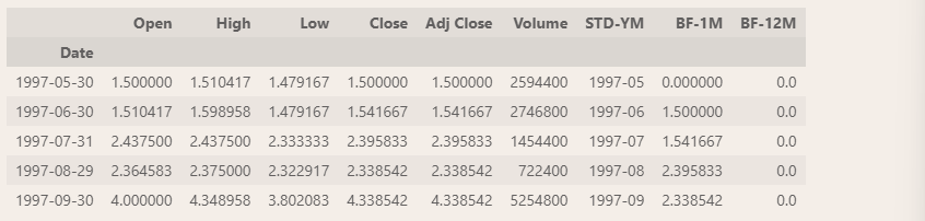
거래 내역 추가
# month_last = 구매 신호(momentum_index)를 확인하기 위함

for i in month_last_df.index:
    signal = ''

    # 절대 모멘텀의 계산식 → (전월의 수정 주가 / 전년의 수정 주가) - 1
    momentum_index = (month_last_df.loc[i, 'BF-1M'] / month_last_df.loc[i, 'BF-12M']) - 1

    # 0보다 크고 무한대가 아닌 경우가 구매 신호
    flag = (momentum_index > 0) & (momentum_index != np.inf)
    if flag:
        signal = 'buy'

    print(f'날짜: {i}, momentum_index: {momentum_index}, signal: {signal}')

    df.loc[i:, 'trade'] = signal
수익률, 누적 수익률 계산
# 수익률, 누적 수익률 계산

df['rtn'] = 1.0

# 수익률 계산
for i in df.index:
    # 매수
    if (df.shift().loc[i, 'trade'] == '') & (df.loc[i, 'trade'] == 'buy'):
        buy = df.loc[i, 'Adj Close']
        print(f"매수일: {i}, 매수가: {buy}")
    elif (df.shift().loc[i, 'trade'] == 'buy') & (df.loc[i, 'trade'] == ''):
        sell = df.loc[i, 'Adj Close']
        rtn = sell / buy
        df.loc[i, 'rtn'] = rtn
        print(f"매도일: {i}, 매도가: {sell}, 수익률: {rtn}")
# 누적 수익률
df['acc_rtn'] = df['rtn'].cumprod()
# 최종 수익률
acc_rtn = df.iloc[-1, -1]

acc_rtn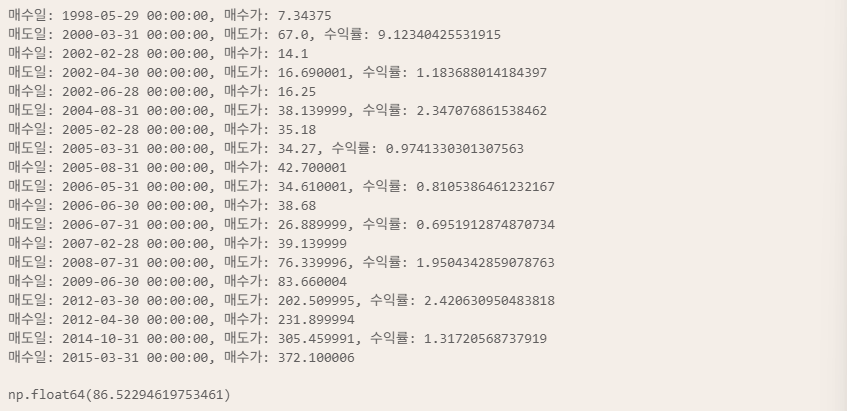
번외: BuyandHold
# byandhold 수익률 계산

buy = df['Adj Close'].iloc[0]
sell = df['Adj Close'].iloc[-1]

print(sell/buy)
	# 974.2744757914
💻 함수화
1. STD-YM 생성 함수
def create_ym(_df, _col = 'Adj Close'):
    df = _df.copy()
    # Date가 column에 포함되어 있는가?
    if 'Date' in df.columns:
        df.set_index('Date', inplace = True)
    df.index = pd.to_datetime(df.index)
    df.index = df.index.tz_localize(None)
    flag = df.isin([np.nan, np.inf, -np.inf]).any(axis=1)
    df = df.loc[~flag, [_col]]
    df['STD-YM'] = df.index.strftime('%Y-%m')

    return df
df = pd.read_csv('../csv/AAPL.csv')
ym_df = create_ym(df)
ym_df.info()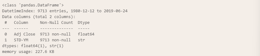
2. 월말 데이터 생성, BF1, BF2 column 생성 함수
def create_month(
        _df,
        _start = '2010-01-01',
        _end = datetime.now(),
        _momentum = 12,
        _last = 1
):

    if _last == 1:
        df = _df.groupby('STD-YM').tail(1)
    elif _last == 0:
        df = _df.groupby('STD-YM').head(1)
    else:
        return "_last 값은 0 또는 1만 가능합니다."

    col = _df.columns[0]

    df['BF1'] = df.shift(1)[col].fillna(0)
    df['BF2'] = df.shift(_momentum)[col].fillna(0)

    df = df.loc[ _start : _end, ]
    return df
month_df = create_month(ym_df)
month_df.head()
3. 거래 내역 추가, 수익률 계산 함수
def create_rtn(_df1, _df2, _score = 1):
    df = _df1.copy()

    df['trade'] = ''
    df['rtn'] = 1.0

    col = df.columns[0]

    # _df2를 이용해서 거래 내역을 생성
    for i in _df2.index:
        signal = ''

        # momentum 계산
        momentum_index = _df2.loc[i, 'BF1'] / _df2.loc[i, 'BF2'] - _score
        flag = (momentum_index > 0) & (momentum_index != np.inf)

        if flag:
            signal = 'buy'

        # 거래 내역 생성
        df.loc[i:, 'trade'] = signal
        print(f'날짜: {i}, momentum_index: {momentum_index}, signal: {signal}')

    # 수익률 계산
    for i in df.index:
        if (df.shift(1).loc[i, 'trade'] == '') & (df.loc[i, 'trade'] == 'buy'):
            buy = df.loc[i, col]
            print(f'매수일: {i}, 매수가: {buy}')
        elif (df.shift(1).loc[i, 'trade'] == 'buy') & (df.loc[i, 'trade'] == ''):
            sell = df.loc[i, col]
            rtn = sell / buy
            df.loc[i, 'rtn'] = rtn
            print(f'매도일: {i}, 매도가: {sell}, 수익률: {rtn}')

    # 누적 수익률 계산
    df['acc_rtn'] = df['rtn'].cumprod()
    acc_rtn = df.iloc[-1, -1]

    return df, acc_rtn
df_final, acc_rtn = create_rtn(ym_df, month_df)
print(acc_rtn)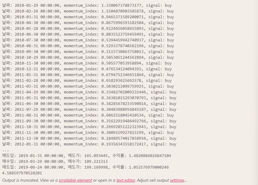
8주차 소감
다음 주 자연어 처리라서 쉬고 가는 타이밍을 만들어주셨는데 벌써부터 걱정된다...🥹
한글이 자연어 처리 중 가장 어렵다고 하는데... 물론 수업은 영어로 할 거지만 괜히 한글 자연어 처리에 대한 욕심이 생겼다고 할까?
원래 아무것도 모를 때 용감하다고 하지... 정신 바짝 차리자🔥
'멀티캠퍼스부트캠프' 카테고리의 다른 글
| 7주차 Note: 머신러닝/딥러닝 (0) | 2026.05.24 |
|---|---|
| 6주차 Note: 머신러닝 (0) | 2026.05.16 |
| 5주차 Note: 머신러닝 (1) | 2026.05.08 |
| 4주차 Note: 데이터 시각화 (0) | 2026.05.01 |
| 3주차 Note: 데이터 수집 (0) | 2026.04.26 |