
5주차: 5월 4일 ~ 5월 8일
멀티캠퍼스 부트캠프 5주차 요약✍️
[ 5/4 ] 휴강
[ 5/5 ] 어린이날 휴강
[ 5/6 ] 시각화: Looker Studio
[ 5/7 ] 머신러닝: Outlier, dummies, 데이터 불균형, 데이터 Split
[ 5/8 ] 머신러닝: 데이터 Scaling, Regression, Classification
5월 6일👩🏻💻
오늘의 소감: Looker는 Tableau와 PowerPoint를 결합한 느낌? UI는 Tableau가 더 예쁘긴 한데, 편의성은 Looker가 조금 더 좋은 듯하다.
둘 모두 시각화 툴이니만큼 크게 차이점이라 할 만한 점은 보이지 않았으니, 두 툴을 함께 공부해도 좋겠다는 생각이 들었다.
수업 시간에 실습한 내용


Tableau는 피벗테이블의 느낌이었다면, Looker는 PPT 만드는 느낌이었달까?
두 툴들의 장점이 명확해서 자유자재로 활용할 수 있다면 정말 나의 분석에 날개를 달아줄 듯한 느낌이 들었다.
5월 7일👩🏻💻
오늘의 소감: 빅분기에서 사용할 수 있는 것들을 많이 배운 날! 시각화가 일찍 끝난 것은 아쉽지만...
학교에서 배웠던 머신러닝을 단단히 다진다 생각하고 열심히 하자!
💻 이상치
wine dataset을 활용한 이상치 처리
라이브러리, 데이터 로드
import pandas as pd
import numpy as np
import matplotlib.pyplot as plt
from sklearn.datasets import load_wine

wine_data = load_wine()
wine = pd.DataFrame(
    data = wine_data['data'],
    columns = wine_data['feature_names']
)
wine['class'] = wine_data['target']

wine
이상치 데이터를 확인
wine.describe()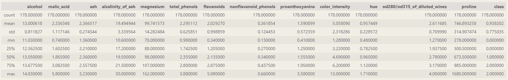
boxplot()
plt.boxplot(wine['color_intensity'])
plt.show()
그래프로 보았을 때 이상치가 4개 정도 보인다.
이상치 필터링
이상치만을 골라내기 위하여 사분위수, IQR을 계산한다.
q_1, q_3 = np.percentile(wine['color_intensity'], [25, 75])
print(q_1)		# 3.2199999999999998
print(q_3)		# 6.2

# IQR 계산
iqr = q_3 - q_1

# 상단 경계 계산
iqr_top = q_3 + 1.5*iqr
# 하단 경계 계산
iqr_bottom = q_1 - 1.5*iqr

print(iqr, iqr_top, iqr_bottom)
# 2.9800000000000004 10.670000000000002 -1.2500000000000009


# 위쪽 이상치 필터링
upper_flag = wine['color_intensity'] > iqr_top
# 아래쪽 이상치 필터링
lower_flag = wine['color_intensity'] < iqr_bottom

wine.loc[upper_flag | lower_flag, ]
이상치 제거, 대체
# 극단치 제거
df = wine.copy()
out_idx = df.loc[upper_flag | lower_flag, ].index
df.drop(out_idx, axis=0)

# 극단치 대체
# 상단의 경계에서 벗어난 데이터는 상단의 경계 값으로 채워주고
# 하단의 경계에서 벗어난 데이터는 하단의 경계 값으로 채워준다.
df2 = wine.copy()
df2.loc[upper_flag, 'color_intensity'] = iqr_top

# 검증용 boxplot
plt.boxplot(df2['color_intensity'])
plt.show()
이상치가 제거된 것을 확인할 수 있다.
💻 범주형 데이터의 변환
더미 변수 생성
# class column의 값들을 범주형으로 변경
wine['class'] = wine['class'].map(
    lambda x: wine_data['target_names'][x]
)

# 더미 변수 생성
dummie_df = pd.get_dummies(wine, columns = ['class'])
dummie_df
💻 데이터의 불균형 해소
샘플링: 다수 데이터와 소수 데이터를 특정 비율로 조절해주는 기법
라이브러리 로드
import pandas as pd
from sklearn.datasets import make_classification
from collections import Counter
from imblearn.under_sampling import RandomUnderSampler
make_classification()
make_classification() : 데이터가 불균형한 랜덤 데이터를 생성
x, y = make_classification(
    n_samples= 1000,
    n_features= 5,
    weights= [0.9],
    flip_y= 0
)

# Counter: 숫자 세는 기능
Counter(y)		# Counter({np.int64(0): 901, np.int64(1): 99})
데이터 프레임으로 엮기
df = pd.DataFrame(x)
df['target'] = y

df.head()
언더 샘플링: RandomUnderSampler()
언더 샘플링: 다수의 라벨을 가진 데이터를 샘플링하여 소수의 데이터의 수준으로 감소시키는 방법
# RandomUnderSampler 라는 class를 생성
undersampler = RandomUnderSampler()

under_x, under_y = undersampler.fit_resample(x, y)

Counter(under_y)		# Counter({np.int64(0): 99, np.int64(1): 99})
undersampler에서 데이터의 비율을 변경
sampling_strategy 매개변수 → 소수 데이터의 비율을 의미, 0.5면 2배
undersampler2 = RandomUnderSampler(sampling_strategy = 0.3)
under_x2, under_y2 = undersampler2.fit_resample(x, y)
Counter(under_y2)		# Counter({np.int64(0): 330, np.int64(1): 99})
오버 샘플링: RandomOverSampler()
오버 샘플링: 소수 데이터를 다수 데이터 개수만큼 증가시켜 학습에 사용하기 위한 방법
랜덤 오버 샘플링: 소수의 데이터를 단순 복제하여 다수의 데이터와의 비율을 맞춰주는 과정
from imblearn.over_sampling import RandomOverSampler
oversampler = RandomOverSampler()
over_x, over_y = oversampler.fit_resample(x, y)
Counter(over_y)		# Counter({np.int64(0): 901, np.int64(1): 901})
# 소수의 데이터 비율을 다수의 반 정도로 샘플링
oversampler2 = RandomOverSampler(sampling_strategy=0.5)
over_x2, over_y2 = oversampler2.fit_resample(x, y)
Counter(over_y2) # Counter({np.int64(0): 901, np.int64(1): 450})오버 샘플링: SMOTE()
SMOTE: 소수 데이터의 관측값에 대한 K개의 최근접 양수를 이웃으로 찾고, 관측 값과 이웃으로 선택된 값 사이에 임의의 새로운 데이터를 생성하는 방법
from imblearn.over_sampling import SMOTE
smote = SMOTE()
sm_x, sm_y = smote.fit_resample(x, y)
Counter(sm_y)		# Counter({np.int64(0): 901, np.int64(1): 901})
SMOTE 결과 시각화
import matplotlib.pyplot as plt
import seaborn as sns

fig, axes = plt.subplots(2, 2, figsize=(15, 15))

# 4개의 산점도 그래프 생성
sns.scatterplot(
    x = x[:, 2], y = x[:, 3], ax = axes[0][0], hue = y, alpha = 0.4
)

sns.scatterplot(
    x = under_x[:, 2], y = under_x[:, 3], ax = axes[0][1], hue = under_y, alpha = 0.4
)

sns.scatterplot(
    x = over_x[:, 2], y = over_x[:, 3], ax = axes[1][0], hue = over_y, alpha = 0.4
)

sns.scatterplot(
    x = sm_x[:, 2], y = sm_x[:, 3], ax = axes[1][1], hue = sm_y, alpha = 0.4
)

axes[0][0].set_title('Origin Data')
axes[0][1].set_title('Random Under Sample')
axes[0][1].set_xlim(-3.5, 3.5)
axes[0][1].set_ylim(-4.5, 4.5)
axes[1][0].set_title('Random Over Sample')
axes[1][1].set_title('SMOTE')

plt.show()
💻 데이터 분할 (Split)
iris dataset을 활용한 이상치 처리
라이브러리, 데이터셋 로드
import pandas as pd
from sklearn.datasets import load_iris
from sklearn.model_selection import train_test_split
iris_data = load_iris()
데이터셋 전처리: 정리, 이상치 처리
iris = pd.DataFrame(iris_data['data'], columns = iris_data['feature_names'])
iris['class'] = iris_data['target']

# target 데이터들의 이름을 변환
iris['class'] = iris['class'].map(
    lambda x: iris_data['target_names'][x]
)

iris
데이터 Split: train_test_split()
X = iris.drop('class', axis=1)
y = iris['class']

X_train, X_test, y_train, y_test = train_test_split(
    X, y, test_size = 0.3, random_state = 42
)

# 데이터의 개수를 확인
print(f'X_train: {X_train.shape}, X_test: {X_test.shape}')
	# X_train: (105, 4), X_test: (45, 4)
print(f'y_train: {y_train.shape}, y_test: {y_test.shape}')
	# y_train: (105,), y_test: (45,)

y_train.value_counts()
train_test_split()의 매개변수
test_size: test 데이터의 비율 (0~1)
random_state: 임의의 데이터를 추출하는 과정에서 seed 값을 지정
shuffle: 데이터를 섞을 것인가(시계열 데이터셋인 경우에는 False)
stratify: 특정 변수를 지정하면 해당 변수를 기준으로 계층화. 해당 변수의 비율을 유지하도록 데이터 분할
X_train2, X_test2, y_train2, y_test2 = train_test_split(
    X, y, test_size = 0.3, shuffle=False, random_state = 42
)

y_train2.value_counts()
X_train3, X_test3, y_train3, y_test3 = train_test_split(
    X, y, test_size = 0.3, stratify=y, random_state=42
)

y_train3.value_counts()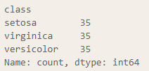
5월 8일👩🏻💻
오늘의 소감:
💻 데이터 Scaling
데이터들의 최솟값과 최댓값, 평균, 표준편차를 출력하는 함수 생성
def scaler_print(train, test):
    print(f"""
    Train Data:
        Min : {round(train.min(), 2)}
        Max : {round(train.max(), 2)}
        Mean: {round(train.mean(), 2)}
        Std : {round(train.std(), 2)}
""")

    print(f"""
    Test Data:
        Min : {round(test.min(), 2)}
        Max : {round(test.max(), 2)}
        Mean: {round(test.mean(), 2)}
        Std : {round(test.std(), 2)}
""")
Standard Scaler
평균이 0, 분산이 1인 정규분포로 스케일링
from sklearn.preprocessing import StandardScaler
stdscaler = StandardScaler()

X_train_sc = stdscaler.fit_transform(X_train3)
X_test_sc = stdscaler.transform(X_test3)
scaler_print(X_train_sc, X_test_sc)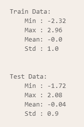
Min-Max Scaler
from sklearn.preprocessing import MinMaxScaler

mnscaler = MinMaxScaler()

X_train_sc = mnscaler.fit_transform(X_train3)
X_test_sc = mnscaler.transform(X_test3)

scaler_print(X_train_sc, X_test_sc)
Max Abs Scaler
from sklearn.preprocessing import MaxAbsScaler
mascaler = MaxAbsScaler()

X_train_sc = mascaler.fit_transform(X_train3)
X_test_sc = mascaler.transform(X_test3)

scaler_print(X_train_sc, X_test_sc)
Robust Scaler
Robust Scaler: 평균과 분산을 이용한 Standard 대신에 중앙값과 사분위수를 활용하는 방식
중앙값을 0으로 설정, IQR을 사용하여 이상치의 영향을 최소화
quantile_range 매개변수(기본값 (25.0, 75.0)): 더 넓거나 좁은 범위의 값을 이상치로 판단하게 할 수 있다.
from sklearn.preprocessing import RobustScaler
ruscaler = RobustScaler()
ruscaler2 = RobustScaler(quantile_range=(20, 80))

X_train_sc = ruscaler.fit_transform(X_train3)
X_test_sc = ruscaler.transform(X_test3)
scaler_print(X_train_sc, X_test_sc)
X_train_sc = ruscaler2.fit_transform(X_train3)
X_train_sc = ruscaler2.transform(X_test3)
scaler_print(X_train_sc, X_test_sc)
inverse_transform
inverse_transform: 스케일링된 데이터를 원본 데이터로 복원
X_origin = ruscaler2.inverse_transform(X_train_sc)
pd.DataFrame(X_origin).head()
💻 회귀 분석
boston dataset을 활용한 회귀 분석
라이브러리, 데이터 로드
import pandas as pd
import matplotlib.pyplot as plt
import seaborn as sns
import numpy as np

from sklearn.model_selection import train_test_split
from sklearn.linear_model import LinearRegression
from sklearn.metrics import r2_score, mean_absolute_error, mean_absolute_percentage_error, \
    mean_squared_error, mean_squared_log_error, root_mean_squared_error

boston = pd.read_csv('../csv/boston.csv')
boston.head()
독립변수, 종속변수 분할 후 데이터 분할
X = boston.drop(columns=['CHAS', 'Price'])
y = boston['Price']

X_train, X_test, y_train, y_test = train_test_split(X, y, test_size = 0.2, random_state = 42)
모델 생성, 학습, 예측
# 모델 생성
lr = LinearRegression()

# 모델 학습
lr.fit(X_train, y_train)

# 예측
pred = lr.predict(X_test)
모델 평가
성능 평가 지표
MAE: | 실제값 - 예측값 |
MSE: MEAN( ( 실제값-예측값 )² )
RMSE: √ MSE
MSLE: log( MSE )
MAPE: MAE %
R² Score: SSR / SST
mae = mean_absolute_error(y_test, pred)
mse = mean_squared_error(y_test, pred)
rmse = root_mean_squared_error(y_test, pred)
mape = mean_absolute_percentage_error(y_test, pred)
r2 = r2_score(y_test, pred)

print(f"MAE: {round(mae, 2)}")				# 3.24
print(f"MSE: {round(mse, 2)}")				# 24.64
print(f"RMSE: {round(rmse, 2)}")			# 4.96
print(f"MAPE: {round(mape, 2)*100}%")			# 17.0%
print(f"R2 Score: {round(r2, 2)}")			# 0.66
💻 분류 분석
iris dataset을 활용한 분류 분석
라이브러리, 데이터 로드
import matplotlib.pyplot as plt
from sklearn.tree import DecisionTreeClassifier, plot_tree
import pandas as pd

iris = pd.read_csv('../csv/iris.csv')
iris.head()
독립변수, 종속변수 분할
X = iris.drop('species', axis=1)
y = iris['species']
모델 생성, 학습, 예측
# 모델 생성
clf = DecisionTreeClassifier(max_depth=3, random_state=42)

# 모델 학습
clf.fit(X, y)
트리 구조 시각화
feature_names = X.columns

plt.figure(figsize=(15, 15))
plot_tree(clf, feature_names=feature_names, class_names=iris['species'].unique(), fontsize=10, filled=True)
plt.show()
train, test 데이터 분할 후 모델 적합, 예측, 평가
# 라이브러리 로드
from sklearn.model_selection import train_test_split
from sklearn.metrics import accuracy_score, confusion_matrix

# 분류 모델이기에 계층화 적용
# split
X_train, X_test, y_train, y_test = train_test_split(
    X, y, test_size=0.2, random_state=42, stratify=y
)

# 모델 적합
clf.fit(X_train, y_train)

# 예측
pred = clf.predict(X_test)

# 평가
accuracy_score(y_test, pred)		# 0.9666666666666667
confusion_matrix(y_test, pred)
# array([[10,  0,  0],
#        [ 0,  9,  1],
#        [ 0,  0, 10]])


# 시각화
plt.figure(figsize=(15, 15))
plot_tree(clf, feature_names=X.columns, class_names=iris['species'].unique(), fontsize=10, filled=True)
plt.show()
5주차 소감
연휴가 있어서 빠르게 지나갔던 5주차!
6주차부터는 본격적인 ML, DL, 자연어 처리를 하게 될 것을 생각하니 새삼 시간이 빠르다.
곧 빅분기 실기 접수도 있으니만큼, 이번에 공부하는 내용들로 sklearn에 대한 지식을 확고히 하자.
저번 시험처럼 linear_model 생각 안 나서 모델 못 쓰지 말고
너무 자동완성에 의존하지 말고, 강사님 따라서 친다고도 생각하지 말고... 내가 내 코드를 건축하는 느낌으로 내것으로 만들자!
'멀티캠퍼스부트캠프' 카테고리의 다른 글
| 7주차 Note: 머신러닝/딥러닝 (0) | 2026.05.24 |
|---|---|
| 6주차 Note: 머신러닝 (0) | 2026.05.16 |
| 4주차 Note: 데이터 시각화 (0) | 2026.05.01 |
| 3주차 Note: 데이터 수집 (0) | 2026.04.26 |
| 2주차 Note: 프로그래밍 기초, 데이터 수집 (0) | 2026.04.26 |